For those of you on Dynamics GP 2013 and later, the SmartList export to Excel has been performance enhanced to make it quicker. In order to gain the increase in speed, the data is sent out as raw text rather than in a table format as in earlier versions. While essentially this doesn’t make much difference, there is definite value for having data in the table.
- Formulas are easier to calculate – no more dragging down the page
- It is much easier to then create a Pivot Table – the range of cells is automatically selected
- If you data size changes – either more or less – the Pivot Table will automatically only look at the relevant data.
Let me tell you how to do it and then I will work through the examples shown above. I am not going to go through all the details for creating a Pivot Table – just the note as to why setting up a table makes it easier.
Export to Excel
The data you export appears as follows:
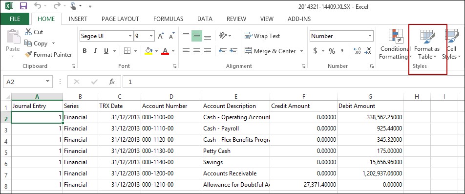
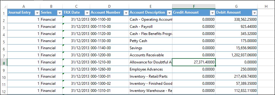
Click on any cell of data. On the “Home” tab, choose to “Format as Table” and choose your style. You will be asked the range of the table and this should default to the full width and length of your data. Click OK and you will see your newly formatted table with filter drop downs at the top.
Adding Formula Columns
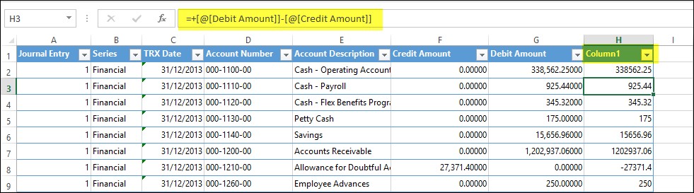
A common calculation to add to exported data is to find the net value of debits and credits (or negate credit notes for AP or AR exports). The usual method is to enter the formula “=G2-F2” in cell H2. You would then drag the formula down to the bottom of the data and add a column heading.
If, after converting to a table, you perform the same action as above, the formula will appear as =+[@[Debit Amount]]-[@[Credit Amount]] and will automatically calculate for all rows in the table. The column will automatically be named “Column1” and can be renamed.
Creating a Pivot Table
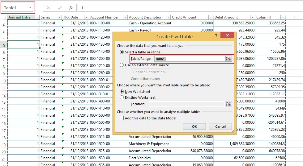
To create a Pivot Table, click on any cell in your table, go to the “Insert” tab and select Pivot Table. The “Create Pivot Table” window appears giving you the opportunity to choose your data range and where you want the Pivot Table to be created.
By having the data in a table, the Table/Range defaults to Table1 (the default name of your new table). This means you are not having to manually select the rows and columns you wish to appear in your Pivot Table selection.
Shrinking Ranges
This would be primarily useful for situations where macros are used to format data after exporting from Dynamics GP (Export Solutions). By formatting at a table, the Pivot Table will automatically be linked to the Table rather than a fixed range of rows and columns.
This is a great tip that I picked up from Belinda Allen’s Creating and Using Excel Pivot Tables session on Virtual Convergence 2014. If you are new to Pivot Tables - or even if like me, you think you are OK with them - I highly recommend this session. I learnt so many other things about Pivot Tables in general - thanks for a fantastic session Belinda.
Heather Roggeveen is a MS Dynamics GP Consultant with Olympic Software. After 15 years of working with the end user all the way from designing the solution to user training, she has become a Dynamics GP expert. Heather regularly shares her knowledge, including tips and tricks for end users in her blog articles. Follow her on Twitter @HRoggeveen to be notified of her latest articles. You can also like Olympic Software on Facebook or follow us on LinkedIn or on Twitter @OlympicSoftware. For more information about Dynamics GP and how it could benefit your business, view the Dynamics GP page on our website or give us a call, 09-357 0022.